Data Analysis on $CO_2$ levels against Tide levels at Labrador Park Costal Trail

About the Author: Year 3 student in National University of Singapore (NUS) in Special Programme in Science

About this Project: Just a small project I did while doing module code SP3175: The Earth with my other groupmates Chua Wei Hong and Joey Cheing

Introduction and Significance

Coastal areas are important ecosystems that bring about multitudes of benefits. Environmentally, coastal areas protect surrounding regions from storms and doubles as a breeding ground for wildlife habitats and commercially important fisheries (Barbier et al., 2011). This in turn, drives the economy by supporting recreation and tourism (McLeod et al., 2011). With the expected increase in sea level, coastal areas are the most vulnerable (Kirwan & Megonigal, 2013). Hence, conservation efforts are imperative. However, before carrying out any conservation plan, we need to have a clear understanding of the carbon balance in coastal areas. Carbon balance in coastal areas is modulated by similar factors upland but there are additional contributions from tidal influences and salinity (Barr et al., 2010). It is important for us to find out the indirect and direct influence of tidal waves on carbon emission at coastal areas. Considering location and tidal patterns, Labrador coastal area stands as an ideal location for the investigation of tidal effects on carbon dioxide emission in Singapore. Hence, our research question: "To investigate the effects of tides on carbon emission at Labrador Nature Reserve.

Data Collection

Location & Sampling Methods

Time-limited systematic samples transec from 1000 - 1200 hours was conducted at Labrador Park Nature Reserve Coastal Trail. Using the 322 equidistant-pillars present along the trail as markers, a random number generator was used to select a random starting point from the first 16 equidistant-pillars. A sampling point was then created after every 16 pillars for a total of 20 sampling points (systematic sampling).

The transects were done at high (water level ≥ 2 m) and low (water level ≤ 1.5 m) tides. Tide times chart for East Coast Park by WindFinder was used to determine the water level at LBNR. A replicate run was done on separate days for each tide type (20th and 21st February 2021 for low tide and 25th and 27th February 2021 for high tide) where the lowest low tide or highest high tide occurred at 1100 hours (± 30 minutes).

Measurement techniques

A Raspberry Pi with K30 10,000ppm $CO_2$ sensor and Adafruit BME280 I2C or SPI Temperature Humidity Pressure Sensor was turned on for two minutes at each sampling point. This was to collect data not only on $CO_2$, but other factors as well such as Humidity and Air Pressure.

Data Analysis

Since the response variable ($CO_2$) is continuous and the explanatory variables are both categorical (High, Low tide levels) and continuous (Temperature, Humidity and Air Pressure, an analysis of covariance (ANCOVA) was performed to determine the significance of the differences in mean $CO_2$ readings.

However, before anything, exploratory plots can be used to infer some key points first before analysis.

All analysis is done in R version 4.1.2.

Results & Discussion

A boxplot of $CO_2$ levels against tide levels was done (below).

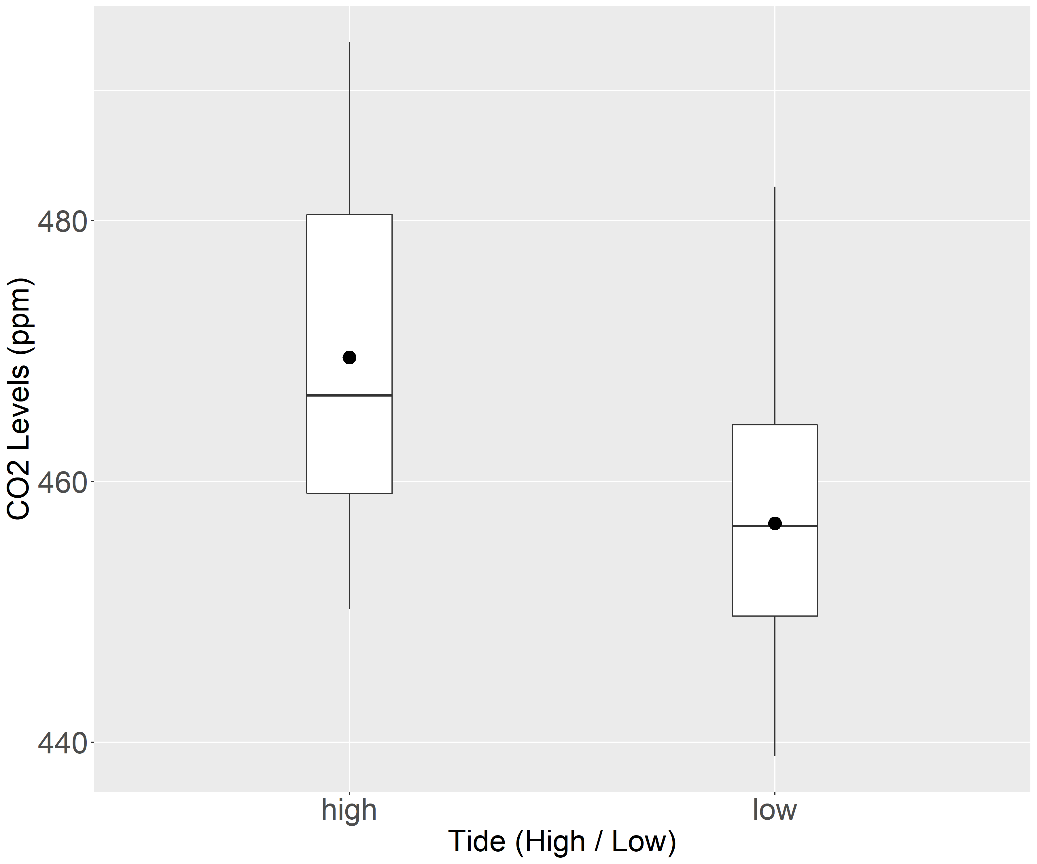co2vsTide Boxplot figure of $CO_2$ levels (ppm) against high and low tides. The blackdots in both boxplots represent the mean whereas the horizontal line represents the median. The mean $CO_2$ for high tide is 459.1ppm, whereas it is 449.7ppm for low tides. First quartile for high tides is 469.5ppm compared to 456.8ppm for low tides and lastly, third quartile of high tides was 480.5ppm as compared to the 464.3ppm of low tides. In order to determine the significance of the differences in two $CO_2$ levels, further analysis needs to be performed

This data indicated that the park had a mean $CO_2$ level of 459.1ppm during high tides compared to the 449.7ppm during low tides. The interquartile range of the $CO_2$ levels are 469.5 - 480.5 ppm for high tide and 456.8 - 464.3 ppm for low tide. However, based of the boxplots alone, we are unable to elaborate on the significance of the two means on a deeper level. In order to investigate the underlying correlations between variables that can explain for the difference in means, the data needs to be further studied using ANCOVA.

Under the ANCOVA framework, multicollinearity tests were conducted and revealed that the interaction term between Humidity and Tide had VIF scores of >3. Furthermore, main effects Temperature and Pressure also had VIF scores of >3. This implied that Humidity and Temperature are linearly correlated with the other explanatory variables present in the model and would then increase the uncertainty of coefficients of the model. Multiple models were compared where no multicollinearity issues were seen using AIC and the model with the lowest AIC was selected. Our final model only had explanatory variables of Humidity and Tide with the lowest AIC. The model was confirmed to be valid as it exhibited homoscedasticity and normaality of its residual from the plot below.

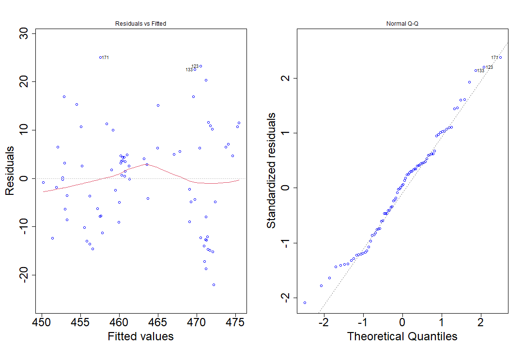Both plots check for the model's assumptions and validity. (Left) The Residuals vs Fitted plot checks for homoscedasticity where the errors are independent. The variance of residuals does not seem to change as fitted values increase, thus confirming homoscedasticity. (Right) The Q-Q plot checks for the normality of the residuals, and in conjunction with Shapiro-Wilk's test (p > 0.05), the residuals are normally distributed.

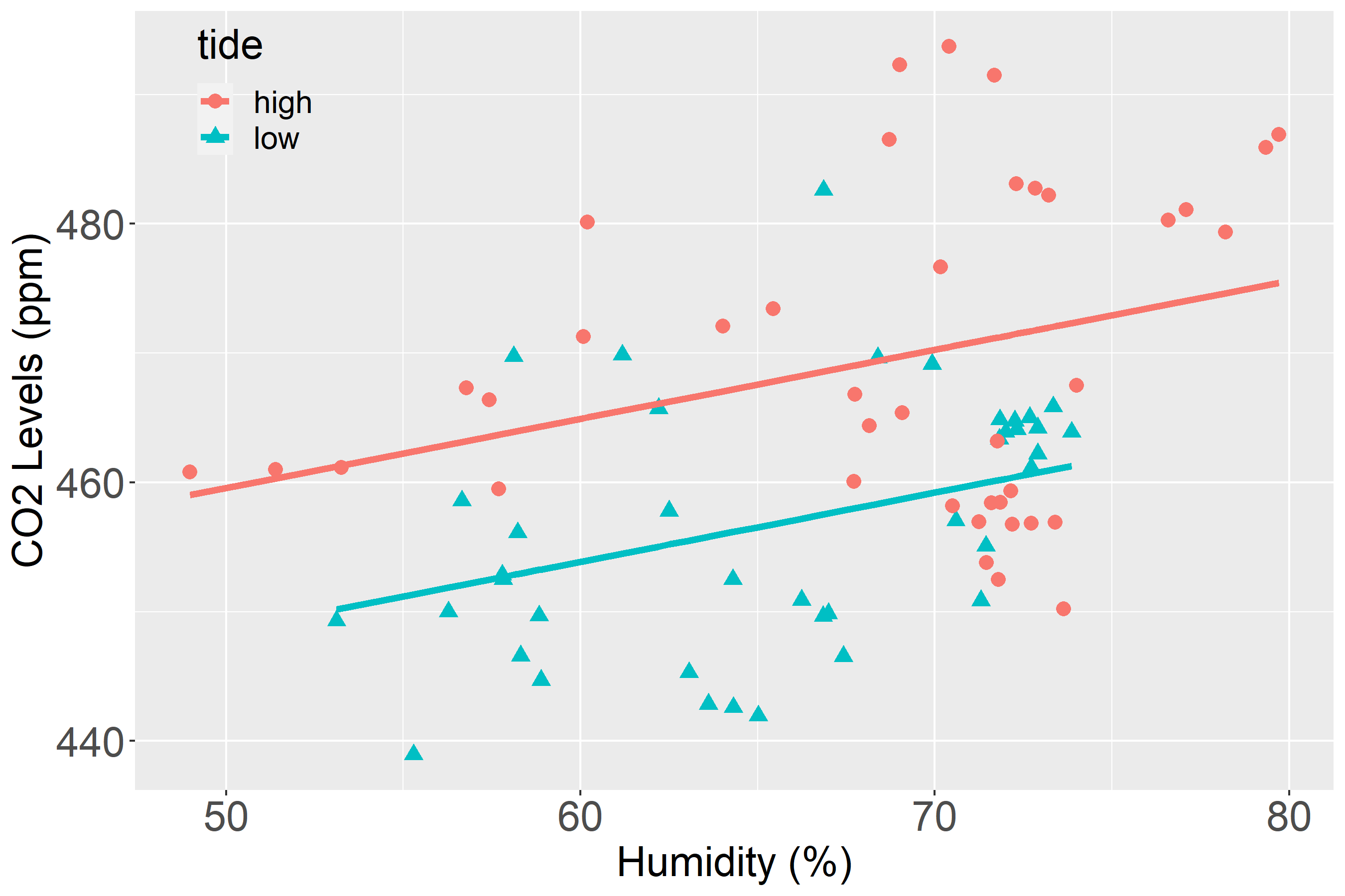
A scatter plot of the various data points were plotted, together with the predicted model fitted values, separated by tide levels in the figure below.

model After correcting for multicollinearity, the model with the lowest AIC score was accepted with the equation $CO_2$ = 0.5304Humidity + 432.842 - 11.046I(Tide = low), $R^2$ = 0.329. The ANCOVA model predicts that $CO_2$ levels at high tides are highter than low tides assuming the same relative Humidity, possibily indicating that the water body is a carbon source. It is important to note that the gradients for $CO_2$ levels at both tides could be different, however it exhibited multicollinearity issues and thus had to be removed from the equation.

Our final model indicated that the relative humidity of the environment is positively correlated with the atmospheric $CO_2$ levels regardless of tide levels and the system can be described with the linear equation:

\[CO_2 = 0.534*Humidity - 11.046*I(Low Tide)\]

This indicated that for every 1% increase in Humidity, it would result in an average increase of 0.534ppm in $CO_2$ level and that the $CO_2$ level would be 11.046ppm higher during high tide than low tide on average, assuming the same relative humidity.

This positive correlation between Humidity and $CO_2$ level may be because humidity is indicative of the amount of water that has evaporated from the nearby water sources. A higher humidity will result in less water to contain dissolved $CO_2$, which in turn increases the amount of dissolved $CO_2$ being released into the air.

The correlation between tide types and $CO_2$ level suggests that the water body at Labrador Nature Reserve Coastal Trail is a carbon source. This is in line with data provided by observatories that analyse temperature of water bodies around the globe. Warm water acts as a carbon source and cold-water acts as a carbon sink. Singapore, situated along the equator, is naturally surrounded by warm water. During high tide, warm water flows throughout the Malayan Peninsula and there will be a surge in the amount of carbon sources at Labrador Nature Reserve Coastal Trail, causing a rise in $CO_2$ levels.

Conclusion

Our study suggested that tide types are significant in influencing $CO_2$ levels at Labrador Nature Reserve. This is attributed to the waters surrounding Singapore being carbon sources. Hence, high water levels (high tide) contributed to a rise in $CO_2$ levels and low water levels (low tide) contributed to a decrease in $CO_2$ levels. Furthermore, relative humidity was found to be positively correlated with atmospheric $CO_2$ levels. Overall, this study is a promising springboard for more comprehensive research on the indirect and direct influence of tidal waves on carbon emission at coastal areas. Coupled with other studieds, meaningful insights can be revealed for the conservation of coastal areas.

Areas of Improvement

Our final model only had an $R^2$ value of 0.329, suggsting that only 32.9% of the observed variances seen in $CO_2$ is explained by the model and the other 67.1% are unexplained. In order to improve the $R^2$ values, known variable that affect $CO_2$ such as water temperature, dissolved $CO_2$ and salinity could have been measured to obtain a model with more explanatory power. A linear mixed effect model could also have been conducted to account for the pseudo-replication as the same route was taken for all measurements, just at different times.

Moreover, $CO_2$ levels could have been measured at East Coast Park so that accurate water levels could have been used as a continuous explanatory response variable. This would allow for a greater understanding of the relationship between $CO_2$ levels, tidal levels and relative humidity.

Data Analysis on \(CO_2\) levels against Tide levels at Labrador Park Costal Trail