Quantitative Model of Honey Bee Colony Population Dynamics
Authors: Darren Teo
About the Authors: Year 3 student in NUS in Special Programme in Science, I am currently majoring in Life Sciences.
About this page: This is essentially a simple project coded in python that explores the paper by Khoury et.al. This page was meant to serve as a sample project for a NUS module SP2273, "Working on Interdisciplinary Science, Pythonically".
A Quantitative Model of Honey Bee Colony Population Dynamics
David S. Khoury, Mary R. Myerscough, Andrew B. Barron
10.1371/journal.pone.0018491
Introduction
Bees are one of the most important species in the ecosystem of our planet. Without them, many flowering plants will be unable to pollinate and eventually die off. This will have resounding effects on many other species that depend on these plants for food and survival.
Beekeepers can tell you how sensitive these little critters are to environmental changes. With the rise of urbanization, deforestation and climate change, bees are facing a massive threat to their existence. However, the significance of the impact due to these factors are not very well understood due to the difficulties in studying these insects.
The paper proposes a simple toy model that can capture the basic dynamics within the hive. The model is independent of the external threat factors, and as such is adaptable for a wide range of studies. The accumulation of external factors that drive the population within the hive can be built upon using this model.
Why study this
In physics and chemistry, when an experiment is repeated over and over again, the same results could be obtained. As a result, mathematical equations can be used to predict the exact results of these experiments.
However in biology, if we repeat the same experiment several times, the results usually are variable. Because of this, it may seem impossible to use mathematical models to predict how a biological system change over time. It turns out, by using mathematical models, we are able to gain insights on the trends of the biological system (even though we are not able to determine the exact results)!
In this paper's context, the authors had also highlighted the importance in modelling a honey bee colony. This is because there is a global decline in bee population and as a result, it was important to check why these colonies are dying out.
Model Equations
The paper took a look at the following model where H is the number of hive bees and F is the number of Forager Bees:
\(\frac{dH}{dt} = E(H,F) - HR(H,F)\) \(\frac{dF}{dt} = HR(H,F) - mF\)
What does the model mean?
Change in Hive bees over time (dH/dt)
The number of hive bees in a given period of time increases based on the Eclosion rate (as denoted by E(H,F)) and this eclosion rate is defined by the number of hive and forager bees.
Then the number of hive bees in a given period of time decreases based on the recruitment function of hive bees to forager bees (as denoted by R(H,F)) and this recruitment rate is also governed by the number of hive and forager bees.
Change in Forager bees over time (dF/dt)
The number of forager bees in a given period of time increases based on the recruitment function of hive bees to forager bees (as denoted by R(H,F)) and this recruitment rate is governed by the number of hive and forager bees.
Then the number of forager bees in a given period of time decreases based on mortality rate faced by Forager bees when they go out of the hive to forage.
Actually defining eclosion function
\[E(H,F) = L(\frac{H+F}{w+H+F})\]The eclosion rate, E(H,F), is governed by the number of Hive and Forager bees over a constant w and egg laying rate L. w is there because it helps to regulate the egg laying rate based on the number of bees in the hive. We can see the effects of this function using the following graph.
# Import Relevant Packages #
import matplotlib.pyplot as plt
import numpy as np
plt.style.use('seaborn')

# Define some constants in our function #
L = 2000
w = 27000

# Define a large range of H+F which I will call N #
Ns = np.arange(10,100000)

#############################################
# Find out what is the function output      #
# based on everything we've defined earlier #
#############################################
Es = L*(Ns/(w + Ns))


# Ploting #
plt.plot(Ns, Es)
plt.xlabel('$H + F$', size = 15)
plt.ylabel('$E(H,F)$', size = 15)
plt.title('Eclosion rate vs Number of Hive (H) and Forager (F) bees', size = 20)
plt.xticks(size = 12)
plt.yticks(size = 12)
plt.show()
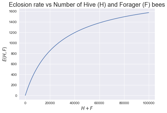
From the graph generated above, it is obvious that as the number of H + F bees increases, the eclosion rate plateaus!
Actually defining recruitment function
\[R(H,F) = \alpha - \sigma(\frac{F}{H+F})\]This function defines the recruitment function of Foragers to Hive bees and Hive bees to Forager bees. We can easily substitute values in to see what this means!
If we assume that there are no Forager bees, we can substitute F = 0, we can see that the recruitment function simplifies to a. This represents the maximum rate that hive bees will become foragers when there are no forager bees present in the colony.
And if we assume that there are significantly more forager bees to hive bees, we can substitute F = infinite and simplify the function to -sigma. This represents how the presence of foragers reduces the rate of recruitment from hive bees to foragers!
As a result the following model is generated:
\[\frac{dH}{dt} = L(\frac{H+F}{w+H+F}) - H(\alpha - \sigma(\frac{F}{H+F}))\] \[\frac{dF}{dt} = H(\alpha - \sigma(\frac{F}{H+F})) - mF\]| Parameter | Estimate | |
|---|---|---|
| \(\alpha\) | 0.25 | |
| \(\sigma\) | 0.75 | |
| \(L\) | 2000 | |
| \(w\) | 27,000 |
Modelling the model
# Import relevant package #
from scipy.integrate import odeint
Using odeint for differential equations
The easiest method to model equations is to use euler's method. However, it has a limitation that the accuracy of the simulation is limited to how small we make the time step (aka dt). We can use a time step small enough to get an accurate simulation but it often comes at a cost of computing power.
Hence, we are going to use odeint instead, which is faster but comes at a cost of not intuitive coding.
The standard odeint function is in this format:
odeint(func,x,t, constants)
funcis your ode function, in our case it is a function to calculate the differential equations (dHdt and dFdt).xrepresents our initial conditions for the model. For our case, the initial number of hive and forager bees.trepresents a list / array of all our time steps being used to calculate.constantsrepresent all the other constants needed in the ode.
Define ode Function
The parameters for the ode function must follow the order as seen in the odeint example showed. Which was x, t, constants. In our case, it would look like ode(x, t, a,sigma,L,w,m).
Oh no, we have 1 input for initial conditions but we have both hive and forager bees to work out! No worries, we would just initialize both in 1 single list! The function needs to then return the values of the differential equation. As a result this would what our function would do in order.
- Unpack
xinto the vario us values of hive and forager bees. This is done by just doingH,F = x[0], x[1] - Calculate the differential equation value by using all the values of H, F and constants.
- Return the differential equations by returning a list
[dhdt, dfdt] - It is important to note that since H is in
x[0]and F is inx[1], the returned list must be[dhdt, dfdt].
def ode(x, t, a, sigma, L, w, m):
    # Unpack
    H,F = x[0], x[1]

    # Calculate
    dhdt = L*(H+F)/(w+H+F) - H*(a - sigma*(F/(H+F)))
    dfdt = H*(a - sigma*(F/(H+F))) - m*F

    # Return the dxdt
    return [dhdt, dfdt]
Define constants
We will first define all the constants defined earlier in the table above. The mortality rate is just set to 0.24 which means 24% of the forager bees would die at every time step.
Since we would want to model what would happen at the start of the colony to the end, the initial hive bees would be 1 and there would be no forager bees. Hence H0, F0 = [1,0].
The time steps was just arbirtually chosen with t = np.linspace(0,1000,200). This function takes in the first value (0) and last value (1000) and generates an array / list that are evenly spaced of a certain length (200).
# Define Constants as stated earlier #
a = 0.25
sigma = 0.75
L = 2000
w = 27000

# Define Mortality Rate #
m = 0.24

# Define the initial conditions for H and F bees #
H0, F0 = [1,0]

# Time steps #
t = np.linspace(0,1000,200)
Putting it all together
x = odeint(ode,[H0, F0],t, (a,sigma,L,w,m))

# We have to split the array that is x into
# our Hs and Fs respectively using slicing
H = x[:,0]
F = x[:,1]

# Plotting Things #
plt.plot(t,H, label = 'Hive Bees')
plt.plot(t,F, label = 'Foraging Bees')
plt.xlabel('Time', size = 15)
plt.ylabel('Number of Bees', size = 15)
plt.xticks(size = 12)
plt.yticks(size = 12)
plt.title(f'Number of Bees over Time with mortality rate: {m}', size = 20)
plt.legend(prop={'size': 15})
plt.show()

Nice, we now have an easy way to model everything and it seems that even if forager bees die at a rate of 24%, the number of bees equilibriate after many years.
Varying the mortality rate of the bees
Now, what would happen if we increase the mortality rate slowly? Let us try m = 0.3 and with the maximum timestep at 2000.
########################
# Define all constants #
########################

# Define Constants as stated earlier #
a = 0.25
sigma = 0.75
L = 2000
w = 27000

# Define Mortality Rate #
m = 0.3 #<---- CHANGE TO 0.3

# Define the initial conditions for H and F bees #
H0, F0 = [1,0]

# Time steps #
t = np.linspace(0,2000,200)

#############
# MODELLING #
#############

x = odeint(ode,[H0, F0],t, (a,sigma,L,w,m))

H = x[:,0]
F = x[:,1]

# Plotting Things #
plt.plot(t,H, label = 'Hive Bees')
plt.plot(t,F, label = 'Foraging Bees')
plt.xlabel('Time', size = 15)
plt.ylabel('Number of Bees', size = 15)
plt.xticks(size = 12)
plt.yticks(size = 12)
plt.title(f'Number of Bees over Time with mortality rate: {m}', size = 20)
plt.legend(prop={'size': 15})
plt.show()
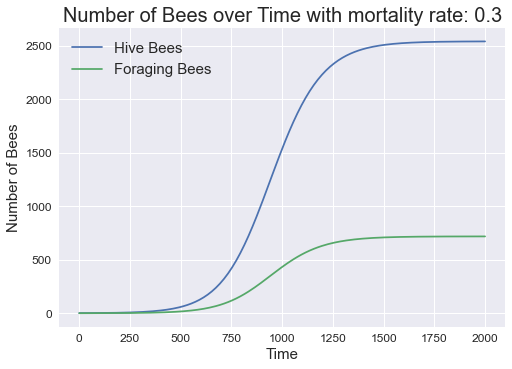
The first thing we noticed is that the colony took longer to equilibriate and the hive and forager bees equilibriate at a lower value as compared to m = 0.24. This is to be expected because more bees are dying and thus the overall number of bees would decline and it will take longer to equilibriate.
Future Works
This analysis of this model is nowhere near complete. There are a few things that we can further explore, some of which include but not limited to:
- Varying the mortality rate of the bees across a wide range to explore the equilibrium value of total bees, hive bees and foraging bees
- Introducing ‘seasons' so that mortality rate of class F bees vary throughout the years (which is what is experienced in real biological systems)
We could continue trying out different levels of mortality rate, but that would be lame. We can use python to do this all for us
Varying mortality rate and plotting them
The simplest plot can be having the y-axis being the equilibriated value and x-axis being the mortality rate. How would we be doing this? Let us break it down for you:
- Using the original model and a certain value of mortality rate, simulate all the way until the number of bees equilibriate
- Taking the last value of the bees in that model and storing them in a list (
F_eqm_lst,H_eqm_lst). - Vary the mortality rate
- Plot the equilibriated values across their respective mortality rate.
########################
# Define all constants #
########################

# Define Constants as stated earlier #
a = 0.25
sigma = 0.75
L = 2000
w = 27000

# Define the initial conditions for H and F bees #
H0, F0 = [1,0]

# Time steps #
t = np.linspace(0,50000,400)


# Generate empty lists for storage
F_eqm_lst, H_eqm_lst = [], []

# Generate a list of mortality rates #
ms = np.arange(0.1, 0.5, 0.0075)

#############
# MODELLING #
#############

for m in ms:
    x = odeint(ode,[H0, F0],t, (a,sigma,L,w,m))
    H = x[:,0]
    F = x[:,1]

    F_eqm_lst.append(F[-1])
    H_eqm_lst.append(H[-1])

plt.plot(ms,H_eqm_lst, 'o' ,label = 'Hive Bees')
plt.plot(ms,F_eqm_lst, 'o' ,label = 'Foraging Bees')
plt.xlabel('mortality rate', size = 15)
plt.ylabel('Number of Bees', size = 15)
plt.title(f'Number of Equilibriated Bees over Mortality rate')
plt.legend()
plt.show()

As expected, we can tell that as mortality rate increases, the number of bees in the colony would naturally decrease. From the graph alone, we can tell that at around m = 0.35, the entire colony would not sustainable and have no bees left.
So what does this tell us?
Around the world, bee colonies might fall due to certain diseases or parasites or competition. However, using these models, the it tells us that the mortality rate of the foragers also directly impacts the entire colony. This can be further linked to the climate issue where the forager bees are exposed to harsher conditions than they can tolerate and thus experience higher mortality which leads to colony collapse!