Histograms
Basic Histogram
First, customary importing of packages and data if you haven't already done so from the previous section.
import pandas as pd
import matplotlib.pyplot as plt

df = pd.read_csv("https://raw.githubusercontent.com/darren1998s/darren1998s.github.io/main/iris.csv")
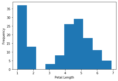
Using the same syntax as the bar chart from the previous section, we can easily plot histograms in the same way.
df['Petal.Length'].plot(kind='hist')

#Don't forget to label your x-axis
plt.xlabel('Petal.Length')
plt.show()
Grouped Histograms
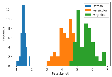
Likewise, like in our previous example, what if we want to check the distribution of Petal.Length grouped by each species of Iris ? We can still make use of the df.groupby() function.
grouped_species = df.groupby("Species")['Petal.Length']
grouped_species.plot(kind='hist')

#Don't forget to enable the legend so we know which colour refers to which species!
plt.legend()

#Don't forget to label your x-axis
plt.xlabel('Petal.Length')
plt.show()
Since we know I. versicolor overlaps with I. virginica, we can set the transparency of the histogram so we can see exactly how they overlap! This can be done by specifying the alpha argument.
grouped_species = df.groupby("Species")['Petal.Length']
grouped_species.plot(kind='hist', alpha = 0.5)

#Don't forget to enable the legend so we know which colour refers to which species!
plt.legend()

#Don't forget to label your x-axis
plt.xlabel('Petal.Length')
plt.show()
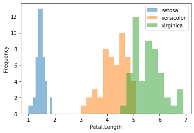
From the histogram above, we can conclude many things on first glance:
-
I. setosa has the lowest mean Petal Length, followed by I. versicolor then I. virginica.
-
The distribution of Petal Length for I. setosa is lower than both I. versicolor and I. virginica.